Finding Evidence for the Environmental Kuznets Curve

Finding Evidence for the Environmental Kuznets Curve

Introduction:

The Kuznets curve was first published in 1955 to describe the relationship between income inequality and per capita income. The shape was an inverted U which proposed that as an economy grows, inequality will increase until it hits a turning point and inequality starts to decrease again. In 1995, Grossman and Krueger first applied the concept of the Kuznets curve to the environment. They found that as an economy grows and until it reaches a per capita income of $8,000, the country will increase it’s pollution. However, after the turning point, that economy will start to lower it’s pollution levels.

Many papers over the years have disputed the existence of the environmental Kuznets curve, including evidence of an N-shaped and inverted N-shape relationship between GDP per capita and carbon dioxide emissions per capita.

First, we examine the relationship between GDP per capita and carbon emissions per capita to determine if there is evidence of an environmental Kuznets curve. For this, we chose 23 different countries in various stages of development and used data that pairs countries by demographics, such as income levels. Here we will examine if countries that are in developing stages are polluting more, while those that are developed are lowering their emissions.

Next, we examine how a carbon cap will affect the economy of a developing nation. The carbon cap will be based on the 1990 level of emissions. Countries will have to end up at a percentage under the 1990 level. By proposing different carbon caps, we can examine the effect of these caps on an economy. We will examine how such an emissions cap will also cap the amount that a nation’s GDP can grow based on the environmental Kuznets Curve theory.

Finally, there is a discussion on how developed nations can bridge the gap of developing nations. Would it be beneficial for developed nations to pay for the alternative energy sources of countries that are affected by the carbon cap? How much should a nation be willing to fund and does that amount depend on the amount of trade a developed country does with a developing nation?

Methodology:

After collecting the data, we made graphs and fit a quadratic line to search for evidence of the Environmental Kuznets Curve. We made a graph for each of the 23 countries and a graph of every country on one plot. Afterwards, we also examined if the trend held based on the development status of countries; i.e. low income vs OECD countries through more graphs.

After seeing a trend in the graphic data we ran regressions using both Pooled OLS and Panel data to observe a relationship between CO₂ emissions and GDP per capita.

Next, we added another covariate, access to alternative energy sources by percentage of the population.

We then looked for a trend between the interaction in the amount of alternative energy available and the GDP to see if the two were dependent on each other. The two following models account for this interaction.

All panel data is grouped by country and set for the year.

Data:

We used three datasets for the analysis, all from the World Bank dataset. Each data set was split into three different groups: Our 23 countries of interest, the various regions data grouped, and data based on a countries demographics. All three are outlined below:

The three data sets used were the GDP per capita of each country / grouping in USD, the carbon dioxide emissions per capita of each country / grouping in metric tons, and the availability of alternative electricity sources of each country / grouping in percent of population with access.

The GDP per capita data sets all the amounts to current USD.

However, the alternative electricity sources per country had less data, so the regression results may have higher standard errors. Without this variable we have 1,357 observations. However, the inclusion of the alternative energy variable drops the number of observations to 1,078. So we look at regressions both with and without the alternative energy variable.

Results:

Graphical evidence of the Kuznets curve:

First, we examine if there is a trend that can be spotted graphically. Each graph will have the data points for emissions and GDP per capita with a quadratic trendline placed over it. Below, there are a couple of graphs to show how the trend may develop for nations in various stages of development.

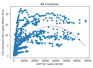
Figure 1: Graph of GDP per Capita and CO₂ Emissions of all data points.

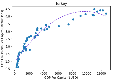
Figure 2: Graph of GDP per Capita and CO₂ Emissions of Turkey (a middle income country) for 1969-2018.

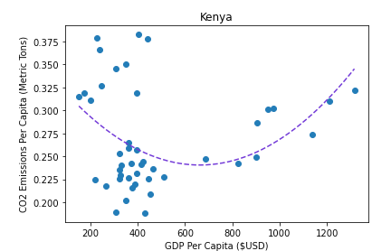
Figure 3: Graph of GDP per Capita and CO₂ Emissions of Kenya (a developing country) for 1969-2018.

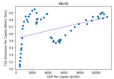
Figure 4: Graph of GDP per Capita and CO₂ Emissions of the World for 1969-2018.

Regression testing for Kuznets curve:

Next, we ran a few separate regressions, as outlined in the methodology section, to look for evidence of the Kuznets curve. From the graphs, there seems to be a third degree trend, so we used GDP₃ in the regression to see if this trend is significant. Below are the results for regressions that don’t use the alternative energy source data.

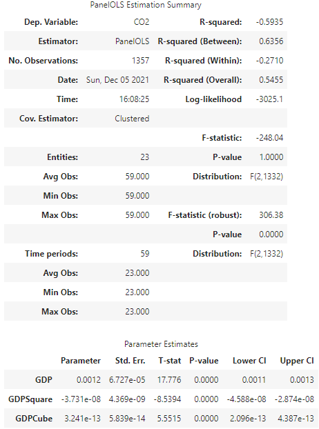
Figure 5: Panel Data Regression of CO₂ on GDP, GDP², and GDP³

The following regression uses the alternative energy data, which had less data points. However, it will show whether access to alternative energy also plays a role in emission outputs, outside of a country’s GDP. There were also interaction terms between GDP and alternative energy to see if there is a significant trend between the two.

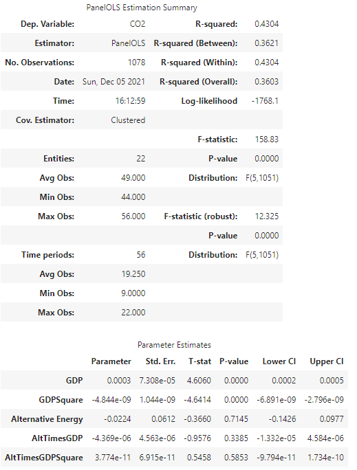
Figure 6: Panel Data Regression of CO₂ on GDP, GDP₂, Alternative Energy, and interaction variables of Alternative Energy with GDP and GDP₂

Discussion:

From our regressions, we find that there is a significant trend between GDP, GDP₂, and GDP₃ even when controlling for access to alternative energy sources. Figure 5 and 6 show, that without any other covariates, GDP is a significant variable for CO₂ emissions. The values of GDP and GDP₂ are evidence of the environmental Kuznets curve. However, there is also a significant third order trend. The negative value for the second order variable and positive for the third order variable give us an N-shaped curve in the data. This is supported by the graphs, especially the graph for World data.

Furthermore, the addition of the access to alternative energy variable does not get rid of the significance of the GDP variable. In these regressions, only GDP and GDP₂ were used to find evidence of an environmental Kuznets curve from the data. From figure 7 and 8, we see that all of the variables, including alternative energy and it’s interaction with GDP are significant variables. However, when using panel data to control for time, we see that the significance of the alternative energy variable drops out.

We can use the original panel data regression with GDP, GDP₂, and GDP₃ to see that there is a significant trend between GDP and CO₂ emission at a third-degree level. Based off of this, we would expect that as GDP rises, CO₂ emissions will also rise up to a point, fall for some time, and then rise again. This trend is supported by our graphs.

Since we found an environmental Kuznets curve trend between GDP and CO₂ emissions, we would like to further this project by implementing a world wide carbon cap which would make countries lower their emissions to 70% of their 1990 levels of emissions. Then, the effects of this carbon cap on the GDP would be examined to determine how much a country’s GDP would be hurt by a cap or how much they would have to spend on alternative energy sources to get back to their old level of energy usage.

We’d also like to explore how other countries could fund the gap and help developing country’s get access to alternative energy sources. It would be worthwhile to explore how the GDP of a developing country can grow when they have access to subsidized alternative energy. Also, it could be beneficial to explore if subsidizing this access will have a net beneficial effect for countries that pay for the alternative electricity sources.

Conclusion:

Based on the regression analysis, there is data to support the environmental Kuznets Curve theory. However, there also seems to be a third degree trend, which can cause an N-shaped curve to form. This means that a country while developing will increase emissions, temporarily lower them, and then raise them again as they continue to develop. We see a third degree trend around a GDP of $1,000 per capita and a slowing of emissions growth around a GDP of $9,000 per capita.